Thermal Transport from HNEMD
Introduction
In this tutorial, we use the HNEMD method to study heat transport in graphene at 300 K and zero pressure. Here we consider the diffusive regime. The ballistic regime can be found in the NEMD example. The spectral decomposition method as described in [Fan 2019] is used here.
Importing Relevant Functions
The inputs/outputs for GPUMD are processed using the Atomic Simulation Environment (ASE).
[16]:
from pylab import *
from ase.build import graphene_nanoribbon
from ase.io import write
from scipy.integrate import cumtrapz
Preparing the Inputs
We consider a graphene sheet of size of about 25 nm x 25 nm (24000 atoms). The transport is in the \(y\) direction. We divide the length in the \(y\) direction into 2 groups, with 4000 atoms in group 0 and 20000 atoms in group 1 We use a Tersoff-style potential (Tersoff (1989)) parameterized by Lindsay et al. [Lindsay 2010].
Generate the model.xyz file:
[7]:
gnr =  graphene_nanoribbon(100, 60, type='armchair', sheet=True, vacuum=3.35/2)
gnr.euler_rotate(theta=90)
l = gnr.cell.lengths()
gnr.cell = gnr.cell.new((l[0], l[2], l[1]))
l = l[2]
gnr.center()
gnr.pbc = [True, True, False]
gnr
[7]:
Atoms(symbols='C24000', pbc=[True, True, False], cell=[245.95121467478057, 255.6, 3.35])
Add Groups
[8]:
Ly = 3*1.42*10
split = [0, Ly, 255.6]

group_label = np.zeros(len(gnr))
for i, atom in enumerate(gnr):
    y_pos = atom.position[1]
    for j in range(len(split)):
        if y_pos > split[j] and y_pos < split[j+1]:
            group_label[i] = j
[9]:
gnr.arrays["group"] = np.array(group_label)
[10]:
for i in range(len(split)-1):
    atom_num = len(gnr[gnr.arrays["group"] == i])
    print(f"group {i}: {atom_num} atoms")
group 0: 4000 atoms
group 1: 20000 atoms
[11]:
write("model.xyz", gnr)
The run.in file:
The run.in input file is given below:
potential    ../../../../potentials/tersoff/Graphene_Lindsay_2010_modified.txt
velocity     300

ensemble     nvt_nhc 300 300 100
time_step    1
dump_thermo  1000
run          1000000

ensemble      nvt_nhc 300 300 100
compute_hnemd 1000 0 0.00001 0
compute_shc   2 250 1 1000 400.0 group 0 0
run           10000000
The first line uses the potential keyword to define the potential to be used, which is specified in the file Graphene_Lindsay_2010_modified.txt.
The second line uses the velocity keyword and sets the velocities to be initialized with a temperature of 300 K.
There are two runs. The first run serves as the equilibration stage.
Here, the NVT ensemble (the Nose-Hoover chain thermostat) is used. The target temperature is 300 K and the thermostat coupling constant is 0.1 ps (100 time steps).
The time_step for integration is 1 fs.
The thermodynamic quantities will be output every 1000 steps.
There are \(10^6\) steps (1 ns) for this run.
The second run is for production.
Here, the global temperature is controlled by the Nose-Hoover chain thermostat (ensemble) with the same parameters as in the equilibration stage.
The compute_hnemd is used to add a driving force and compute the thermal conductivity using the HNEMD method [Fan 2019]. Here, the conductivity data will be averaged for each 1000 steps before written out, and the driving force parameter is \(10^{-5}\) A-1 and is in the \(y\) direction.
The line with the compute_shc keyword is used to compute the spectral heat current (SHC). The SHC will be calculated for group 0 in grouping method 0. The relevant data will be sampled every 2 steps and the maximum correlation time is \(250 \times 2 \times 1~{\rm fs} = 500~{\rm fs}\). The transport directions is 1 (\(y\) direction). The number of frequency points is 1000 and the maximum angular frequncy is 400 THz.
There are \(10^7\) steps (10 ns) in the production run. This is just an example. To get more accurate results, we suggest you use \(2 \times 10^7\) steps (20 ns) and do a few independent runs and then average the relevant data.
Results and Discussion
Computation Time
Using a GeForce RTX 2080 Ti GPU, the HNEMD simulation takes about 1.5 hours.
Figure Properties
[12]:
aw = 2
fs = 16
font = {'size'   : fs}
matplotlib.rc('font', **font)
matplotlib.rc('axes' , linewidth=aw)

def set_fig_properties(ax_list):
    tl = 8
    tw = 2
    tlm = 4

    for ax in ax_list:
        ax.tick_params(which='major', length=tl, width=tw)
        ax.tick_params(which='minor', length=tlm, width=tw)
        ax.tick_params(which='both', axis='both', direction='in', right=True, top=True)
Plot HNEMD Results
The kappa.out output file is loaded and processed to create the following figure.
[14]:
labels_kappa = ['kxi', 'kxo', 'kyi', 'kyo', 'kz']
kappa_array = np.loadtxt("kappa.out")

kappa = dict()
for label_num, key in enumerate(labels_kappa):
    kappa[key] = kappa_array[:, label_num]
[17]:
def running_ave(y, x):
    return cumtrapz(y, x, initial=0) / x

t = np.arange(1,kappa['kxi'].shape[0]+1)*0.001  # ns
kappa['kyi_ra'] = running_ave(kappa['kyi'],t)
kappa['kyo_ra'] = running_ave(kappa['kyo'],t)
kappa['kxi_ra'] = running_ave(kappa['kxi'],t)
kappa['kxo_ra'] = running_ave(kappa['kxo'],t)
kappa['kz_ra'] = running_ave(kappa['kz'],t)
[18]:
figure(figsize=(12,10))
subplot(2,2,1)
set_fig_properties([gca()])
plot(t, kappa['kyi'],color='C7',alpha=0.5)
plot(t, kappa['kyi_ra'], linewidth=2)
xlim([0, 10])
gca().set_xticks(range(0,11,2))
ylim([-2000, 4000])
gca().set_yticks(range(-2000,4001,1000))
xlabel('time (ns)')
ylabel(r'$\kappa_{in}$ W/m/K')
title('(a)')

subplot(2,2,2)
set_fig_properties([gca()])
plot(t, kappa['kyo'],color='C7',alpha=0.5)
plot(t, kappa['kyo_ra'], linewidth=2, color='C3')
xlim([0, 10])
gca().set_xticks(range(0,11,2))
ylim([0, 4000])
gca().set_yticks(range(0,4001,1000))
xlabel('time (ns)')
ylabel(r'$\kappa_{out}$ (W/m/K)')
title('(b)')

subplot(2,2,3)
set_fig_properties([gca()])
plot(t, kappa['kyi_ra'], linewidth=2)
plot(t, kappa['kyo_ra'], linewidth=2, color='C3')
plot(t, kappa['kyi_ra']+kappa['kyo_ra'], linewidth=2, color='k')
xlim([0, 10])
gca().set_xticks(range(0,11,2))
ylim([0, 4000])
gca().set_yticks(range(0,4001,1000))
xlabel('time (ns)')
ylabel(r'$\kappa$ (W/m/K)')
legend(['in', 'out', 'total'])
title('(c)')


subplot(2,2,4)
set_fig_properties([gca()])
plot(t, kappa['kyi_ra']+kappa['kyo_ra'],color='k', linewidth=2)
plot(t, kappa['kxi_ra']+kappa['kxo_ra'], color='C0', linewidth=2)
plot(t, kappa['kz_ra'], color='C3', linewidth=2)
xlim([0, 10])
gca().set_xticks(range(0,11,2))
ylim([0, 4000])
gca().set_yticks(range(-2000,4001,1000))
xlabel('time (ns)')
ylabel(r'$\kappa$ (W/m/K)')
legend(['yy', 'xy', 'zy'])
title('(d)')

tight_layout()
show()
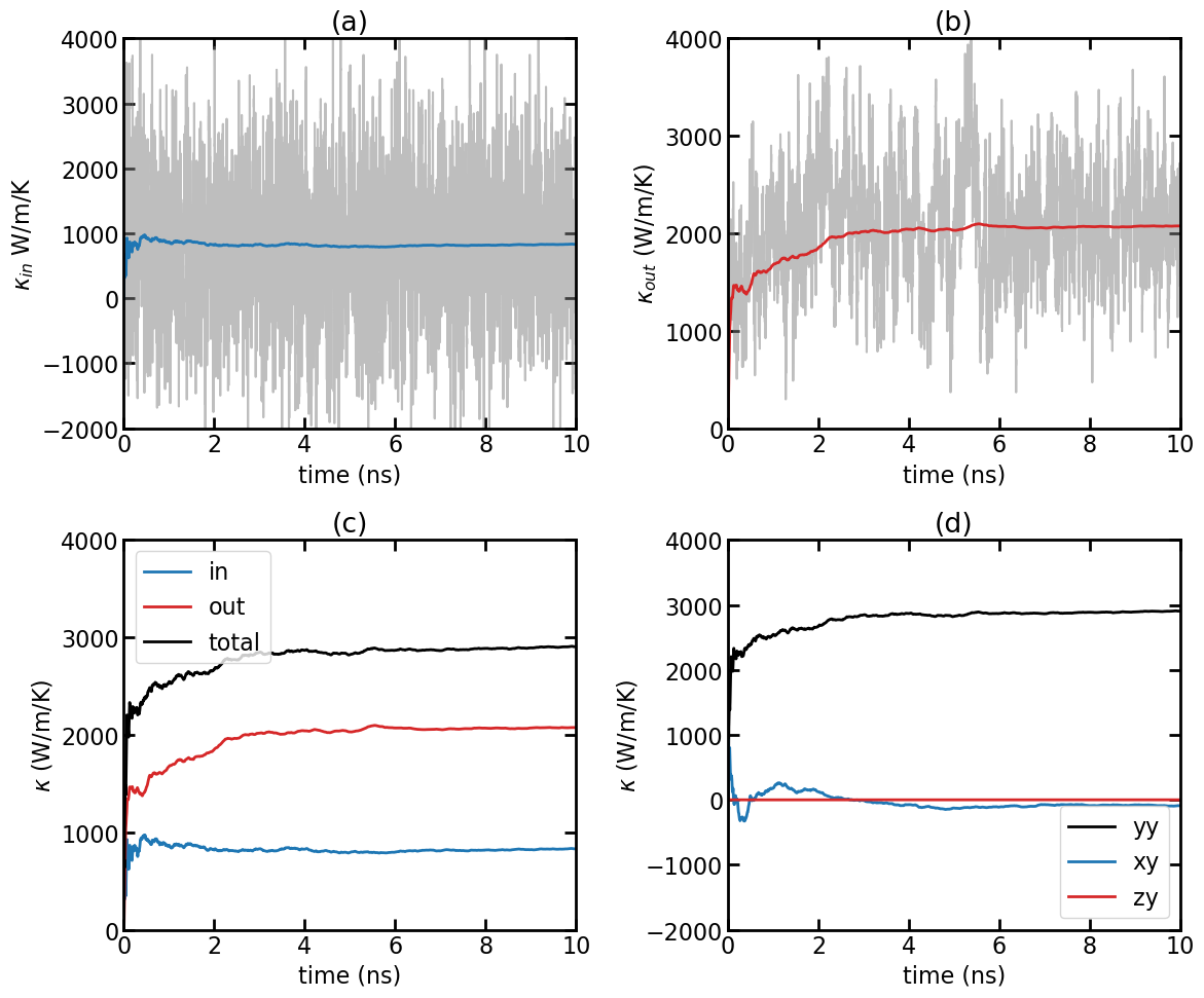
(a) In-plane thermal conductivity \(\kappa_{\rm in}(t)\) as a function of production time. (b) Out-of-plane thermal conductivity \(\kappa_{\rm out}(t)\) as a function of production time. (c) In-plane, out-of-plane, and total thermal conductivity as a function of production time. (d) Comparing \(\kappa_{yy}\), \(\kappa_{xy}\), and \(\kappa_{zy}\).
The gray line represents the instant in-plane thermal conductivity \(\kappa_{\rm in}(t)\) from the kappa.out file. The dashed line represents the cumulative time average:
\[\kappa^{\rm ave}_{\rm in}(t) = \frac{1}{t} \int_0^t \kappa_{\rm in}(t') dt'\]
Similar to (a), but for the out-of-plane thermal conductivity \(\kappa_{\rm out}(t)\) and \(\kappa^{\rm ave}_{\rm out}(t)\).
Cumulative time averaged in-plane, out-of-plane, and total thermal conductivity: \(\kappa^{\rm ave}_{\rm in}(t)\), \(\kappa^{\rm ave}_{\rm out}(t)\) and \(\kappa^{\rm ave}_{\rm total}(t) = \kappa^{\rm ave}_{\rm in}(t) + \kappa^{\rm ave}_{\rm out}(t)\). It is clear that the out-of-plane phonons have a much large average phonon relaxation time (scattering time) than the in-plane phonons, and the thermal conductivity in pristine graphene is dominated by out-of-plane (flexural) phonons. This is consistent with the results from the EMD simulation as discussed in the EMD tutorial.
Some cumulative time averaged thermal conductivity components of the tensor: \(\kappa^{\rm ave}_{yy}(t)\), \(\kappa^{\rm ave}_{xy}(t)\) and \(\kappa^{\rm ave}_{zy}(t)\). It is clear that the off-diagonal components of the thermal conductivity tensor are zero.
Plot Spectral Heat Current Results
The shc.out output file is loaded and processed to create the following figure.
[19]:
num_corr_points, num_omega = 250, 1000

labels_corr = ['t', 'Ki', 'Ko']
labels_omega = ['omega', 'jwi', 'jwo']

num_corr_points_in_run = num_corr_points * 2 - 1
coor_array = np.loadtxt("shc.out", max_rows=num_corr_points_in_run)
omega_array = np.loadtxt("shc.out", skiprows=num_corr_points_in_run)

shc = dict()
for label_num, key in enumerate(labels_corr):
    shc[key] = coor_array[:, label_num]

for label_num, key in enumerate(labels_omega):
    shc[key] = omega_array[:, label_num]
shc["nu"] = shc["omega"] / (2*np.pi)

shc.keys()
[19]:
dict_keys(['t', 'Ki', 'Ko', 'omega', 'jwi', 'jwo', 'nu'])
[21]:
def calc_spectral_kappa(shc, driving_force, temperature, volume):
    # ev*A/ps/THz * 1/A^3 *1/K * A ==> W/m/K/THz
    convert = 1602.17662
    shc['kwi'] = shc['jwi'] * convert / (driving_force * temperature * volume)
    shc['kwo'] = shc['jwo'] * convert / (driving_force * temperature * volume)


l = gnr.cell.lengths()
Lx, Lz = l[0], l[2]
V = Lx * Ly * Lz
T = 300
Fe = 1.0e-5
calc_spectral_kappa(shc, driving_force=Fe, temperature=T, volume=V)
shc['kw'] = shc['kwi'] + shc['kwo']
shc['K'] = shc['Ki'] + shc['Ko']
Gc = np.load('Gc.npy')
shc.keys()
[21]:
dict_keys(['t', 'Ki', 'Ko', 'omega', 'jwi', 'jwo', 'nu', 'kwi', 'kwo', 'kw', 'K'])
[22]:
lambda_i = shc['kw']/Gc
length = np.logspace(1,6,100)
k_L = np.zeros_like(length)
for i, el in enumerate(length):
    k_L[i] = np.trapz(shc['kw']/(1+lambda_i/el), shc['nu'])
[23]:
figure(figsize=(12,10))
subplot(2,2,1)
set_fig_properties([gca()])
plot(shc['t'], shc['K']/Ly, linewidth=3)
xlim([-0.5, 0.5])
gca().set_xticks([-0.5, 0, 0.5])
ylim([-1, 5])
gca().set_yticks(range(-1,6,1))
ylabel('K (eV/ps)')
xlabel('Correlation time (ps)')
title('(a)')

subplot(2,2,2)
set_fig_properties([gca()])
plot(shc['nu'], shc['kw'],linewidth=3)
xlim([0, 50])
gca().set_xticks(range(0,51,10))
ylim([0, 200])
gca().set_yticks(range(0,201,50))
ylabel(r'$\kappa$($\omega$) (W/m/K/THz)')
xlabel(r'$\nu$ (THz)')
title('(b)')

subplot(2,2,3)
set_fig_properties([gca()])
plot(shc['nu'], lambda_i,linewidth=3)
xlim([0, 50])
gca().set_xticks(range(0,51,10))
ylim([0, 6000])
gca().set_yticks(range(0,6001,1000))
ylabel(r'$\lambda$($\omega$) (nm)')
xlabel(r'$\nu$ (THz)')
title('(c)')

subplot(2,2,4)
set_fig_properties([gca()])
semilogx(length/1000, k_L,linewidth=3)
xlim([1e-2, 1e3])
ylim([0, 3000])
gca().set_yticks(range(0,3001,500))
ylabel(r'$\kappa$ (W/m/K)')
xlabel(r'L ($\mu$m)')
title('(d)')

tight_layout()
show()
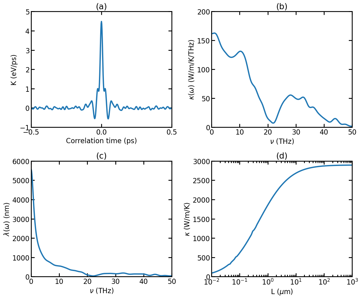
(a) Virial-velocity correlation function \(K(t)\). (b) Spectral thermal conductivity \(\kappa(\omega)\). (c) Spectral phonon mean free path \(\lambda(\omega)\). (d) Length-dependent thermal conductivity \(\kappa(L)\).
The above figure shows the results from the HNEMD simulation [Fan 2019].
The virial-velocity correlation function \(K(t)\). See Theoretical formulations for the definition of this quantity.
The spectral thermal conductivity \(\kappa(\omega)\). See Theoretical formulations for the definition of this quantity.
The spectral phonon mean free path calculated as [Fan 2019]
\[\lambda(\omega)=\kappa(\omega)/G(\omega),\]where \(G(\omega)\) is the quasi-ballistic spectral thermal conductance from the above NEMD simulation.
The length-dependent thermal conductivity calculated as [Fan 2019]
\[\kappa(L) = \int \frac{d\omega}{2\pi} \frac{\kappa(\omega)}{1 + \lambda(\omega)/L}.\]
References
[Fan 2019] Zheyong Fan, Haikuan Dong, Ari Harju, and Tapio Ala-Nissila, Homogeneous nonequilibrium molecular dynamics method for heat transport and spectral decomposition with many-body potentials, Phys. Rev. B 99, 064308 (2019).
[Lindsay 2010] L. Lindsay and D.A. Broido, Optimized Tersoff and Brenner emperical potential parameters for lattice dynamics and phonon thermal transport in carbon nanotubes and graphene, Phys. Rev. B, 81, 205441 (2010).
[Tersoff 1989] J. Tersoff, Modeling solid-state chemistry: Interatomic potentials for multicomponent systems, Phys. Rev. B 39, 5566(R) (1989).