Constructing a NEP model

Introduction

In this tutorial, we will show how to use the nep executable to train a NEP potential and check the results. For background on the NEP approach see this section of the documentation.

Prerequisites

You need to have access to an Nvidia GPU with compute capability >= 3.5. CUDA 9.0 or higher is also needed to compile the GPUMD package. You can download GPUMD, unpack it, go to the src directory, and type make -j to compile. Then, you should get two executables: gpumd and nep in the src directory.

Train a NEP potential for PbTe

To train a NEP potential, one must prepare at least two input files: train.xyz and nep.in. The train.xyz file contains all the training data, and the nep.in file contains some controlling parameters. One can also optionally provide a test.xyz file that contains all the testing data.

Prepare the train.xyz and test.xyz files

• The train.xyz/test.xyz file should be prepared according to the documentation.

• For the example in this tutorial, we have already prepared the train.xyz and test.xyz files in the current folder, which contain 25 and 300 structures, respectively.

• In this example, there are only energy and force training data. In general, one can also have virial training data.

• We used the VASP code to calculate the training data, but nep does not care about this. You can generate the data in train.xyz/test.xyz using any method that works for you. For example, before doing new DFT calculations, you can first check if there are training data publicly available and then try to convert them into the format as required by train.xyz/test.xyz. There are quite a few tools (https://github.com/brucefan1983/GPUMD/tree/master/tools) available for this purpose.

Prepare the nep.in file.

• First, study the documentation about this input file.

• For the example in this tutorial, we have prepared the nep.in file in the current folder.

• The nep.in file reads:

type         2 Te Pb

This is the simplest nep.in file, with only one keyword, which means that there are \(N_{\rm typ}=2\) atom types in the training set: Te and Pb. The user can also write Pb first and Te next. The code will remember the order of the atom types here and record it into the NEP potential file nep.txt. Therefore, the user does not need to remember the order of the atom types here. All the other parameters will have good default values (please check the screen output).

Run the nep executable

• Go to the current folder from command line and type

path/to/nep # linux
path\to\nep # Windows

It took about 12 minutes to run 10,000 generations using my laptop with a GeForce RTX 2070 GPU card. One can kill the executable at any time and also restart it by simply running the executable again.

Check the training results

• After running the nep executable, there will be some output on the screen. We encourage the user to read the screen output carefully. It can help to understand the calculation flow of nep.

• Some files will be generated in the current folder and will be updated every 100 generations (some will be updated every 1000 generations). Therefore, one can check the results even before finishing the maximum number of generations as set in nep.in.

• If the user has not studied the documentation of the output files generated by nep, it is time to read about those here.

• We will use Python to visualize the results in some of the output files next. We first load pylab that we need.

from pylab import *

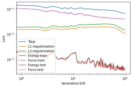
Checking the loss.out file

• We see that the \(\mathcal{L}_1\) and \(\mathcal{L}_2\) regularization loss functions first increases and then decreases, which indicates the effectiveness of the regularization.

• The energy loss is the root mean square error (RMSE) of energy per atom, which converges to about 0.4 meV/atom.

• The force loss is the RMSE of force components, which converges to about 40 meV/Å.

loss = loadtxt('loss.out')
loglog(loss[:, 1:6])
loglog(loss[:, 7:9])
xlabel('Generation/100')
ylabel('Loss')
legend(['Total', 'L1-regularization', 'L2-regularization', 'Energy-train', 'Force-train', 'Energy-test', 'Force-test'])
tight_layout()

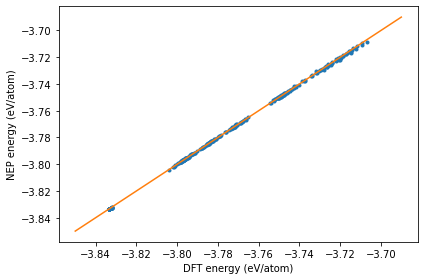
Checking the energy_test.out file

The dots are the raw data and the line represents the identity function used to guide the eyes.

energy_test = loadtxt('energy_test.out')
plot(energy_test[:, 1], energy_test[:, 0], '.')
plot(linspace(-3.85,-3.69), linspace(-3.85,-3.69), '-')
xlabel('DFT energy (eV/atom)')
ylabel('NEP energy (eV/atom)')
tight_layout()

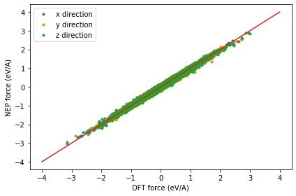
Checking the force_test.out file

The dots are the raw data and the line represents the identity function used to guide the eyes.

force_test = loadtxt('force_test.out')
plot(force_test[:, 3:6], force_test[:, 0:3], '.')
plot(linspace(-4,4), linspace(-4,4), '-')
xlabel('DFT force (eV/A)')
ylabel('NEP force (eV/A)')
legend(['x direction', 'y direction', 'z direction'])
tight_layout()

Checking the virial_test.out file

In general, one can similarly check the virial_test.out file, but in this particular example, virial data were not used in the training process (no virial data exist in train.xyz/test.xyz).

Checking the other files

One can similarly check the other files: energy_train.out, force_train.out, and virial_train.out.

Restart

• After each 100 steps, the nep.restart file will be updated.

• If nep.restart exists, it means you want to continue the previous training. Remember not to change the parameters related to the descriptor and the number of neurons. Otherwise the restarting behavior is undefined.

• If you want to train from scratch, you need to delete nep.restart first (better to first make a copy of all the results from the previous training).