Constructing a NEP polarizability model
Introduction
In this tutorial, we will show you how to use the GPUMD package to train a NEP polarizability model and analyze the results. For theoretical background on the NEP approach, please read the documentation. A paper that introduces the NEP polarizability model systematically is in preparation.
Prerequisites
You need to have access to an NVIDIA GPU with compute capability >= 3.5. Besides it, CUDA Toolkit 9.0 or higher is needed to compile the GPUMD package. The latest GPUMD (we recommend v3.7 or newer) can be downloaded here. Unpack it, go to the src directory, and run the command make -j to compile. If success, you should get two executables: gpumd and nep in the src directory. The flag “-std=c++14” in makefile can be modified
to “-std=c++11” if you failed the compilation process.
Train a NEP polarizability model for QM7B database
To train a NEP polarizability model, two files: train.xyz and nep.in are mandatory. The train.xyz file contains necessary training data, and the nep.in file contains some parameters used for training. Optionally, one can also provide a test.xyz file that has similar contents as thetrain.xyz for validation.
Prepare the train.xyz and test.xyz files
The
train.xyz/test.xyzfile should be prepared according to the documentation.In this tutorial,
train.xyzandtest.xyzfiles are already prepared in the current folder, which contain 5768 and 1443 structures, respectively. Structures as well as polarizability data in thetrain.xyzandtest.xyzare taken from the QM7B database that contains 7211 organic compounds. The (static) polarizability is a symmetric second-order tensor that has a form of\[\begin{split}\boldsymbol{\alpha }=\left( \begin{matrix} \alpha _{xx}& \alpha _{xy}& \alpha _{xz}\\ \alpha _{yx}& \alpha _{yy}& \alpha _{yz}\\ \alpha _{zx}& \alpha _{zy}& \alpha _{zz}\\ \end{matrix} \right)\end{split}\]The polarizability data are embedded in the comment lines of
train.xyz/test.xyz, organized as *pol=” \(\alpha _{xx}\) $:nbsphinx-math:alpha `*{xy} $ :math:alpha _{xz}` \(\alpha _{yx}\) $:nbsphinx-math:alpha `*{yy} $ :math:alpha _{yz}` \(\alpha _{zx}\) $:nbsphinx-math:alpha `_{zy} $ :math:alpha _{zz}`”* per structure. The polarizability data were computed at the CCSD/d-aug-cc-pVDZ level of theory by Yang and collaborators. Of course, you can use any quantum mechanics package and any theoretical method such as the DFT to calculate the polarizability. However, structures in QM7B database are without lattice information, which is mandatory in the training of NEP models. Therefore, a cubic box with a dimension of 100 \(\rm \mathring{A}\) was set for every structure. We recommend the ASE package to manipulate thetrain.xyz/test.xyzfile.
Prepare the nep.in file.
First, read the documentation regarding input paramaters carefully. The most important parameter is
model_type, which controls the training types.model_type=0which is default, stands for a training task of PES;model_type=1, a training task of dipole;model_type=2, a training task of polarizability. Here, we setmodel_type=2. A minimalnep.infile reads:
type        6 H C N O S Cl
model_type        2
The parameter type is also important, which specified the element kinds in the system. The first value 6 is the number of elements in train.xyz/test.xyz, followed by the detailed element names, in this case, H C N O S Cl. The order will be frozen in the model after training. We have prepared the nep.in file in the current folder, which reads:
type         6 H C N O S Cl
model_type         2
cutoff       6 4
n_max        6 6
basis_size    10 10
l_max        4 2 1
neuron       10
population    80
batch        10000
generation   200000
lambda_1     0.03
lambda_2     0.03
The values of parameters cutoff, n_max,basis_size,l_max, neuron,population used here were tested elaborately, which achieved a good balance between the accuracy and costs. The batch size depends on your GPU device. On a GeForce RTX 3090 with 24 GB memory, you can train the model with all data at the same time, therefore, we set batch a value greater than 5768. The lambda_1 and lambda_1 are the regularization
paramaters. You can take the default values trustingly just ignore these two parameters. The GPUMD will adjust these two parameters dynamically according to the real-time loss. Alternatively, you can set lambda_1 and lambda_2 a fixed value which should be of the same order as the target quantities upon convergence. In this example, we set lambda_1=lambda_2=0.03.We
will look back on it after analyzing the results.
Run the nep executable
Run the following command in the working directory
path/to/nep # if you use linux
path\to\nep # if you use Windows
It took about 22 hours to run 200,000 generations using a GeForce RTX 3090. One can kill the task at any time and also restart it just by running the nep again.
Check the training results
After you launch the
neptask, there should be some output on the screen. We encourage the user to read the screen output carefully. It can help to understand the working flow ofnep.Some files will be generated in the current folder and will be updated every 100 generations (some will be updated every 1000 generations). Therefore, one can check the results even before finishing the maximum number of generations as set in
nep.in.If the user has not read the documentation regarding the output files, it is time to read about those here.
We will use Python to visualize the results in some of the output files next. We first load
pylabthat we need.
[2]:
from pylab import *
Checking the loss.out file
We see that the \(\mathcal{L}_1\) and \(\mathcal{L}_2\) regularization loss functions first increases and then decreases, which indicates the effectiveness of the regularization.
The polarizability loss is the root mean square error (RMSE) of polarizability per atom, which converges to about 0.03-0.04 a.u./atom.
[3]:
loss = loadtxt('loss.out')
loglog(loss[:, 1:4])
loglog(loss[:, 4:6])
xlabel('Generation/100')
ylabel('Loss')
legend(['Total', 'L1-regularization', 'L2-regularization', 'Polarizability-train', 'Polarizability-train'])
tight_layout()
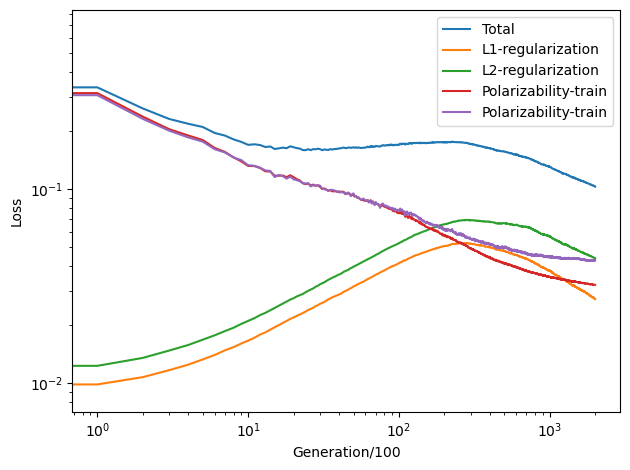
The loss terms ‘Polarizability-train’ and ‘Polarizability-train’ converged after 20,000 generations (But you can run it longer). That’s why we choose the paramaters lambda_1=lambda_2=0.03. But you can take the default values trustingly.
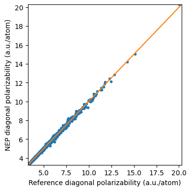
Checking the polarizability_test.out file
The polarizability_test.out is organized as “\(\alpha _{xx}\) $:nbsphinx-math:alpha `*{yy} $ :math:alpha _{zz}` \(\alpha _{xy}\) $:nbsphinx-math:alpha `*{yz} $ :math:alpha _{xz}` \(\alpha _{xx}\) $:nbsphinx-math:alpha `*{yy} $ :math:alpha _{zz}` \(\alpha _{xy}\) $:nbsphinx-math:alpha `*{yz} $ :math:alpha _{xz}`”, one line per structure. The first six values are predicted by NEP, while the last six values are the references we provide in
test.xyz(but divided by the number of atoms).
[6]:
# for diagonal elements
pol_diag_test = loadtxt('polarizability_test.out',usecols=(0,1,2,6,7,8))
ref_values = np.hstack([pol_diag_test[:,3],pol_diag_test[:,4],pol_diag_test[:,5]])
nep_values = np.hstack([pol_diag_test[:,0],pol_diag_test[:,1],pol_diag_test[:,2]])
plot(ref_values,nep_values , '.')
plot(linspace(pol_diag_test.min(),pol_diag_test.max()), linspace(pol_diag_test.min(),pol_diag_test.max()), '-')
xlim((pol_diag_test.min(),pol_diag_test.max()))
ylim((pol_diag_test.min(),pol_diag_test.max()))
xlabel('Reference diagonal polarizability (a.u./atom)')
ylabel('NEP diagonal polarizability (a.u./atom)')
fig = plt.gcf()
fig.set_size_inches(4,4)
tight_layout()
[7]:
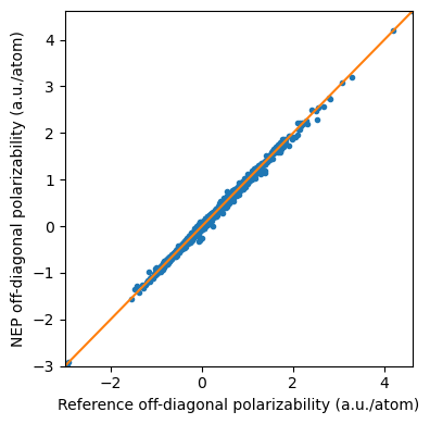
# for off-diagonal elements
pol_offdiag_test = loadtxt('polarizability_test.out',usecols=(3,4,5,9,10,11))
ref_values = np.hstack([pol_offdiag_test[:,3],pol_offdiag_test[:,4],pol_offdiag_test[:,5]])
nep_values = np.hstack([pol_offdiag_test[:,0],pol_offdiag_test[:,1],pol_offdiag_test[:,2]])
plot(ref_values,nep_values , '.')
plot(linspace(pol_offdiag_test.min(),pol_offdiag_test.max()), linspace(pol_offdiag_test.min(),pol_offdiag_test.max()), '-')
xlim((pol_offdiag_test.min(),pol_offdiag_test.max()))
ylim((pol_offdiag_test.min(),pol_offdiag_test.max()))
xlabel('Reference off-diagonal polarizability (a.u./atom)')
ylabel('NEP off-diagonal polarizability (a.u./atom)')
fig = plt.gcf()
fig.set_size_inches(4,4)
tight_layout()
Get molecular polarizability
Numbers of atoms are varied for different structures in the QM7B database. To get their polarizability, we should know their numbers of atoms. The following Python script can be used to obtain the molecular polarizability for each structure in test.xyz.
[16]:
import os
file_size = os.path.getsize("test.xyz")
noa_list = []
with open("test.xyz") as reader:
    while (reader.tell() < file_size):
        noa = int(reader.readline())
        noa_list.append(noa)
        for i in range(noa+1):
            reader.readline()

atomic_pol_diag_test = loadtxt('polarizability_test.out',usecols=(0,1,2,6,7,8))

molecular_diagonal_polarizability = atomic_pol_diag_test * np.tile(np.array(noa_list).reshape(-1,1),(1,6))
print("Diagonal elements:")
print(molecular_diagonal_polarizability)

atomic_pol_offdiag_test = loadtxt('polarizability_test.out',usecols=(3,4,5,9,10,11))

molecular_offdiag_polarizability = atomic_pol_offdiag_test * np.tile(np.array(noa_list).reshape(-1,1),(1,6))
print("Off-diagonal elements:")
print(molecular_offdiag_polarizability)
Diagonal elements:
[[ 86.93239  81.89478  64.59779  86.77072  81.95972  63.94601]
 [ 66.87154  75.06843  70.12993  67.42251  75.463    70.00906]
 [ 95.30625  72.51928  69.21652  95.10905  72.87611  68.8432 ]
 ...
 [ 65.3233   67.70946  55.286    65.57978  67.49064  55.38372]
 [ 78.4861  118.855    47.02907  77.48224 119.3984   47.36193]
 [ 68.6895   70.45695  68.69175  68.29755  70.4676   68.9577 ]]
Off-diagonal elements:
[[-2.1363730e+00 -2.0750540e+00  7.9340360e+00 -1.8626050e+00
  -1.8792140e+00  7.2918270e+00]
 [ 1.8631660e+00  1.6867077e+00  8.0070000e-01  2.1008430e+00
   1.8908760e+00  6.6708000e-01]
 [ 1.4109745e+01  3.6405840e+00  1.7375190e+00  1.4100157e+01
   3.8441590e+00  1.6899003e+00]
 ...
 [ 6.9831720e-01 -1.1632208e+00  6.2205360e+00  9.8580300e-01
  -9.8249060e-01  6.4980860e+00]
 [ 3.3778140e+01 -6.1842220e-02  2.8229300e-02  3.3851840e+01
  -8.4909000e-02  2.3642960e-02]
 [-1.2690855e-01  9.5440650e-02 -8.6488950e+00 -1.1436195e-01
   9.4393050e-02 -8.2682400e+00]]
Prediction
You can switch the workding mode from training to prediction by adding an extra parameter
prediction 1innep.in, and provide atrain.xyz. In this mode, the polarizability data is not necessary intrain.xyz. TheNEPwill use-1e+06as the reference values inpolarizability_train.out. We also provide an example in theprediction_new_moleculedirectory.
Restart
After each 100 steps, the
nep.restartfile will be updated.If
nep.restartexists, it means you want to continue the previous training. Remember not to change the parameters related to the descriptor and the number of neurons. Otherwise the restarting behavior is undefined.If you want to train from scratch, you need to delete
nep.restartfirst (better to first make a copy of all the results from the previous training).
Author
Nan Xu
[ ]: